Diabetes 130 US hospitals for years 1999-2008 / 당뇨병 환자가 30일 이내에 병원을 재방문 할 것인지에 대한 인공지능 예측(2)

지난글에 이어서 모델 학습 및 평가를 시작하겠습니다. 

 

사용할 모델입니다.
- LogisticRegression
- RandomForest
- DecisionTree

#- GridSearchCV -
GridSearchCV는 최적의 파라미터를 찾아주고 교차검증도 해줍니다.
여기서 파라미터란 모델에서 bias 값 즉 예측할때 가장 적합한 값을 찾아준다고 보면됩니다.
y = wX+b 에서 b값이라고 보면됩니다.

#- SMOTE -
y의 값이 불균형적이라 1의 값을 늘리고 0의 값을 줄이고 하는 복합적으로 불균형한 데이터를 균형있게
맞출 수 있도록 SMOTE를 씁니다. SMOTE는 데이터를 늘리고 줄여서 데이터를 변화시키기 때문에
반드시 train 데이터셋에만 적용합니다. test값은 실제로 테스트해봐야하기 때문에 그데로 보존
하여야 합니다.

 

from sklearn.linear_model import LogisticRegression
from sklearn.tree import DecisionTreeClassifier
from sklearn.ensemble import RandomForestClassifier
from sklearn.model_selection import GridSearchCV
from imblearn.over_sampling import SMOTE

def fitClasifiers(gs_clfs, X, y):
    for clf in gs_clfs:
        print(X.shape)
        clf.fit(X, y)

def showGridsearchResult(gs_clfs):
    estimators = []
    scores = []
    params = []

    for clf in gs_clfs:
        estimators.append(str(clf.estimator))
        scores.append(clf.best_score_)
        params.append(clf.best_params_)

    for i, val in enumerate(estimators):
        print(val)
        print(scores[i])
        print(params[i])

X_train, X_test, y_train, y_test = train_test_split(X_Scaled, y, test_size=0.2, stratify=y)

# 모델설정
sm = SMOTE(random_state=42)

# SMOTE under sampling
X_train, y_train = sm.fit_resample(X_train, y_train)

lr = LogisticRegression()
dt = DecisionTreeClassifier()
rf = RandomForestClassifier()

param_lr = {"penalty": ["l2"]}
param_tree = {"max_depth": [3, 4, 5, 6], "min_samples_split": [2, 3]}

gs_lr = GridSearchCV(lr, param_grid=param_lr, cv=5, refit=True)
gs_dt = GridSearchCV(dt, param_grid=param_tree, cv=5, refit=True)
gs_rf = GridSearchCV(rf, param_grid=param_tree, cv=5, refit=True)

gs_clfs = [gs_lr, gs_dt, gs_rf]

fitClasifiers(gs_clfs, X_train, y_train.values.ravel())
showGridsearchResult(gs_clfs)

 

위의 결과는 acc 확률 입니다.

LogisticRegression acc : 61.1%

DecisionTreeClassifier acc : 82.6%

RandomForestClassifier : 81.9%

나왔습니다. 

from sklearn.metrics import accuracy_score, confusion_matrix, roc_auc_score
from sklearn.metrics import recall_score, precision_score, roc_curve
from sklearn.metrics import precision_recall_curve

def showMetrics(y_test, y_pred):
    confusion = confusion_matrix(y_test, y_pred)
    accuracy = accuracy_score(y_test, y_pred)
    precision = precision_score(y_test, y_pred)
    recall = recall_score(y_test, y_pred)
    print(confusion)
    print("Acc : {}".format(accuracy))
    print("precision : {}".format(precision))
    print("recall : {}".format(recall))

def showPrecisionRecallCurve(y_test, prob_positive_pred):
    precisions, recalls, thresholds = precision_recall_curve(y_test, prob_positive_pred)
    print("th val : {}".format(thresholds[:4]))
    print("precision val : {}".format(precisions[:4]))
    print("recalls val : {}".format(recalls[:4]))

    df = {
        "thresholds": thresholds,
        "precisions": precisions[:-1],
        "recalls": recalls[:-1]
    }
    df = pd.DataFrame.from_dict(df)

    sns.lineplot(x="thresholds", y="precisions", data=df)
    sns.lineplot(x="thresholds", y="recalls", data=df)
    plt.show()

def showRocCurve(y_test, prob_positive_pred):
    fpr, tpr, thresholds = roc_curve(y_test, prob_positive_pred)

    print("fpr val : {}".format(fpr[:4]))
    print("tpr val : {}".format(tpr[:4]))
    print("thresholds val : {}".format(thresholds[:4]))

    df = {"threshold": thresholds, "fpr": fpr, "tpr": tpr}
    df = pd.DataFrame.from_dict(df)
    sns.lineplot(x="fpr", y="tpr", data=df)
    plt.show()

    roc_score = roc_auc_score(y_test, prob_positive_pred)
    print("roc_score : " + str(roc_score))

print('##################################')
print('###### LogisticRegression ########')
print('##################################')

y_pred = gs_lr.predict(X_test)
pred_prob = gs_lr.predict_proba(X_test)
print("### LogisticRegression show_metrics ###")
showMetrics(y_test, y_pred)

y_pred = np.concatenate([pred_prob, y_pred.reshape(-1, 1)], axis=1)
prob_positive_pred = y_pred[:, 1]
print("### LogisticRegression showPrecisionRecallCurve ###")
showPrecisionRecallCurve(y_test, prob_positive_pred)

print("### LogisticRegression showRocCurve ###")
showRocCurve(y_test, prob_positive_pred)

print(' \n')
print(' \n')

print('##################################')
print('######### RANDOM FOREST ##########')
print('##################################')

y_pred = gs_rf.predict(X_test)
pred_prob = gs_rf.predict_proba(X_test)
print("### RANDOM FOREST showMetrics ###")
showMetrics(y_test, y_pred)

y_pred = np.concatenate([pred_prob, y_pred.reshape(-1, 1)], axis=1)
prob_positive_pred = y_pred[:, 1]
print("### RANDOM FOREST showPrecisionRecallCurve ###")
showPrecisionRecallCurve(y_test, prob_positive_pred)

print("### RANDOM FOREST showRocCurve ###")
showRocCurve(y_test, prob_positive_pred)

print(' \n')
print(' \n')

print('##################################')
print('######### DecisionTree ###########')
print('##################################')

y_pred = gs_dt.predict(X_test)
pred_prob = gs_dt.predict_proba(X_test)
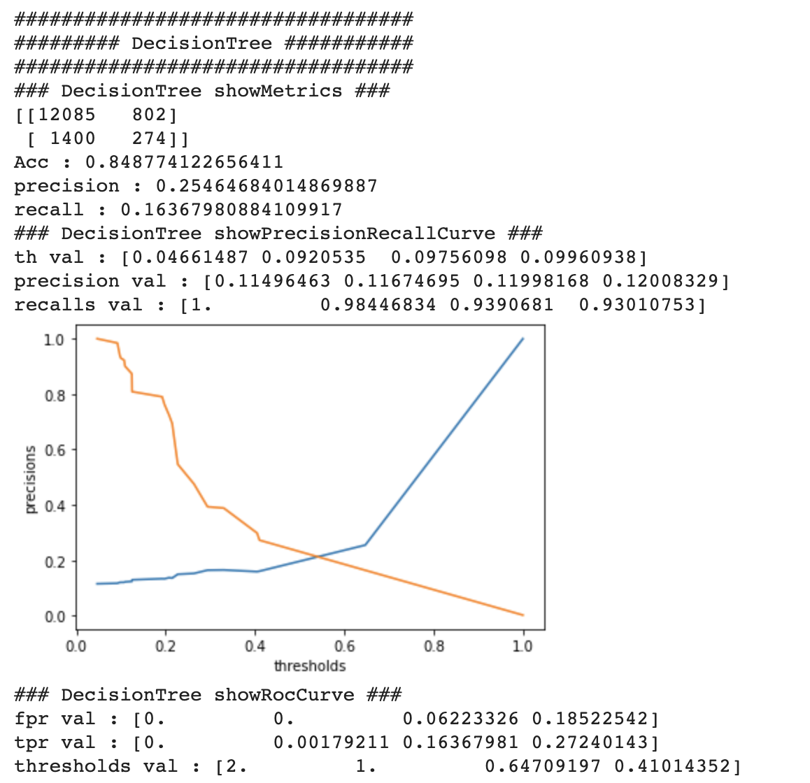
print("### DecisionTree showMetrics ###")
showMetrics(y_test, y_pred)

y_pred = np.concatenate([pred_prob, y_pred.reshape(-1, 1)], axis=1)
prob_positive_pred = y_pred[:, 1]
print("### DecisionTree showPrecisionRecallCurve ###")
showPrecisionRecallCurve(y_test, prob_positive_pred)

print("### DecisionTree showRocCurve ###")
showRocCurve(y_test, prob_positive_pred)

결과표 해석하는법 입니다. 

-- 예제 --

### show_metrics ###
[[79 10]
[24 33]]
Acc : 0.7671232876712328
precision : 0.7674418604651163
recall : 0.5789473684210527

# 위의 결과에서
    0   1
0 79 10
1 23 33

79 + 10 + 23 + 33 = 145 (test data 총 갯수 )

79: TN(true negative) / 실제 값이 0(negative)인데 0이라고 맞춘 갯수
10 : FN(false negative) / 실제 값이 0(negative)인데 1이라고 틀린 갯수
23: FP(false positive) / 실제 값이 1(positive)인데 0이라고 틀린 갯수
33 : TP(true positive) / 실제 값이 1(positive)인데 1이라고 맞춘 갯수

Acc는 전체 145개에서 79+33 맞춘 퍼센테이지이고
precision은 TP/(FP+TP)이며 33/(23+33) 입니다.
헬스케어 데이터에서는 질병이 걸렸느냐 안걸렸느냐, 이번 데이터에서는 30일 이내에 재방문 했느냐 안했느냐가 중요합니다.
따라서 1의 값을 얼마나 잘 맞추었냐가 더 중요합니다. 1의 값을 맞춘 비율이 precision입니다.

Acc로 판단했을때의 위험요소는 만약 1000개의 데이터에서 900개가 0이고 100개가 1일때(inbalance data)
1을 맞추지 않고 전부 0이라고 예측해버리면 90퍼센트의 정확도가 나오기 때문에 Acc로 판단하기는 위험합니다.

recall은 TP/(FN+TP)이며 1이라고 예측한 값들 중에 10과 33이 있으며 이중에서 얼마나 질병이 걸렸는지
잘 예측했는지 보는 결과입니다. 33/(10+33)

 

#- showPrecisionRecallCurve -
th val : [0.04994261 0.06008972 0.0710064 0.07128134]
precision(정확도) val : [0.44186047 0.4375 0.44094488 0.43650794]
recalls(재현율) val : [1. 0.98245614 0.98245614 0.96491228]

precisions, recall : 결론적으로 acc값보다 precision과 recall값이 더 의미가 있으며 모델 평가에 있어서 중요합니다.

 

# - showRocCurve -

* fpr : false positive rate
* tpr : true positive rate
* tpr = recall

thresholds :
thresholds를 만약 0.3으로 정했다면 예측값은 확률로 나오는데 만약 질병이 걸렸다고 예측하는 확률이
0.4라면 질병이 걸렸다고 1이라고 값을 반환합니다. 즉 thresholds는 걸렸다 안걸렸다를 확실하게 구분해주는
기준치라고 보면됩니다.

그럼 thresholds가 1이라면 당연히 0.99의 확률로 병에 걸렸다고 예측하여도 0의 값이 나옵니다.
show_precision_recall_curve의 그래프 교차지점의 thresholds의 값이 가장 적합한 기준치라고 봐도됩니다.

roc 커브는 이런 다양한 모델 평가 부분들을 한눈에 볼 수 있는 그래프 입니다. 30일 이내에 재방문하는 사람을
30일 이내에 재방문 할것이라고 예측하고 그렇지 않은 사람을 재방문 하지 않을 것이라고 예측하는 것이
tpr = 1 이고 fpr = 0이 되는 것입니다.

결국 roc 커브에서 모델의 평가가 좋다는 것은 커브의 밑면적 즉 auc의 넓이가 넓을수록 성능이 좋습니다.
roc_score값이 결국 예측을 얼마나 잘 했느냐입니다.

---------------------------------------------------------------------------

---------------------------------------------------------------------------

 

 

 

LogisticRegression의 roc score가 62%로 가장 높게 나왔습니다.

이번 학습에서는 60%대의 모델 성능이 나왔는데
첫째로, y label 의 불균형 문제가 심하여 그럴 수 있습니다. 이 경우에는 under sampling, over sampling,
under-over sampling(복합샘플링) 방법들을 사용하여 y label 의 균형을 어느정도 맞춰 볼 수가 있습니다.(물론 이 방법들을 사용하셔도 해결이 되지 않을 수 있습니다),
y의 0 값을 가진 행들을 삭제하는 방법이 under sampling 의 일종이라고 볼 수 있겠습니다.

다음의 레퍼런스 사이트를 한번 참고해 보시면 도움이 될 것 같습니다.
불균형클래스 처리를 위한 4가지 방법 설명 https://dining-developer.tistory.com/27
SMOTE 를 통한 데이터 불균형처리 https://mkjjo.github.io/python/2019/01/04/smote_duplicate.html

둘째로, Logistic Regression 과 같은 모델의 경우, 변수들의 수가 많아지면 성능의 저하가 일어날 수 있습니다.

셋째로, Kaggle에서 다른분들이 해놓으신것을 찾아보았으나 auc가 60%인건 마찬가지인것 같습니다. 데이터 자체가
60%를 넘기가 힘들수도 있습니다.
https://medium.com/analytics-vidhya/diabetes-130-us-hospitals-for-years-1999-2008-e18d69beea4d
AUC_RF = 0.6633526103243218